Deep-learning-based single-domain and multidomain protein structure prediction with D-I-TASSER

Substantial progress in protein three-dimensional (3D) structure prediction has been witnessed by the community-wide critical assessment of protein structure prediction (CASP) experiments^1,2. A first milestone in the field occurred when deep learning was used to predict local structure features³, such as contact and distance maps^4,5,6, hydrogen bonding⁷ and torsion/dihedral angles⁸, and full-length 3D models was then constructed by optimally satisfying the geometry predictions, typically through quasi-Newton minimization⁹ followed by full-atom relax¹⁰ or the crystallography and nuclear magnetic resonance system¹¹. Another wave of predictions is led by an end-to-end learning protocol, AlphaFold2 (ref. ¹²), which was developed to further improve the two-stage restraint-based modeling methods. Most recently, AlphaFold3 (ref. ¹³) found that the effectiveness and generality of the end-to-end learning can be further enhanced by the integration of the diffusion samples. These deep learning approaches demonstrated more accurate performance over the traditional structural folding methods built on extensive physical force field-based simulations, such as I-TASSER^14,15, Rosetta¹⁰ and QUARK¹⁶. Although physics-based methods retain their use for studying protein folding principles and pathways, such as through tracking simulation trajectories, the CASP results raised an important question about the necessity and usefulness of physics-based approaches to high-accuracy protein structure prediction¹⁷.

Furthermore, an important existing limitation in the field is that most advanced methods emphasize the modeling of domain-level structures, which constitute the fundamental folding and functional units within the complicated protein tertiary structures. Nevertheless, two-thirds of prokaryotic proteins and four-fifths of eukaryotic proteins incorporate multiple domains¹⁸ and execute higher-level functions through domain–domain interactions¹⁹. Most methods for modeling multidomain proteins, including both physics and deep-learning-based approaches, lack a multidomain processing module^20,21. Consequently, the accurate and efficient modeling of multidomain proteins remains a challenge in the field.

We present a hybrid pipeline, deep-learning-based iterative threading assembly refinement (D-I-TASSER), which couples multisource deep learning features, including contact/distance maps and hydrogen-bonding networks, with cutting-edge iterative threading assembly simulations²² for atomic-level protein tertiary structure modeling. Different from the quasi-Newton minimization algorithm, which requires the differentiability of the objective function, Monte Carlo simulations performed by D-I-TASSER allow for the implementation of the full version physics-based force field of I-TASSER for structural optimization and refinement when coupled with the deep learning models. In addition, a new domain-splitting and reassembly module is introduced for the automated modeling of large multidomain protein structures. Both benchmark tests and the most recent blind CASP15 experiment showed that the hybrid D-I-TASSER pipeline surpasses traditional I-TASSER series methods and outperforms the state-of-the-art deep learning approaches AlphaFold2 (ref. ¹²) and AlphaFold3 (ref. ¹³). As an illustration of large-scale application, D-I-TASSER was applied to the structural modeling of the entire human proteome and resulted in a larger coverage of foldable sequences compared to the recently released AlphaFold Structure Database²³. The D-I-TASSER programs and the genome-wide modeling results have been made freely accessible to the community through https://zhanggroup.org/D-I-TASSER/. All benchmark datasets and the standalone package are available at https://zhanggroup.org/D-I-TASSER/download/ for academic use.

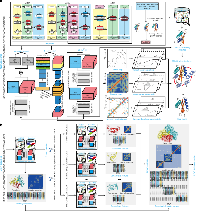
D-I-TASSER is designed for hybrid deep learning and threading fragment assembly-based protein structure modeling with a focus on nonhomologous and multidomain proteins. As shown in Fig. 1a, D-I-TASSER first constructs deep multiple sequence alignments (MSAs) by iteratively searching genomic and metagenomic sequence databases and selects the optimal MSA through a rapid deep-learning-guided prediction process. The pipeline then creates spatial structural restraints by DeepPotential^7,24,25, AttentionPotential and AlphaFold2 (ref. ¹²), which are driven by deep residual convolutional, self-attention transformer and end-to-end neural networks, respectively. Full-length models are then constructed by assembling template fragments from multiple threading alignments by LOcal MEta-Threading Server (LOMETS3)²⁶ through replica-exchange Monte Carlo (REMC) simulations²⁷, under the guidance of a highly optimized deep learning and knowledge-based force field. To tackle the complexity of multidomain structural modeling, D-I-TASSER incorporated a new domain partition and assembly module, in which domain boundary splitting, domain-level MSAs, threading alignments and spatial restraints are created in an iterative mode, where the multidomain structural models are created by full-chain I-TASSER assembly simulations as guided by the hybrid domain-level and interdomain spatial restraints (Fig. 1b). A detailed description of the D-I-TASSER pipeline, including force fields and various protocols, is given in the Methods.

Benchmark of D-I-TASSER on single-domain proteins

Structural modeling of single-domain proteins is fundamental for computational protein structure prediction. To examine the performance of our pipeline, we first tested D-I-TASSER on a set of 500 nonredundant ‘Hard’ domains collected from the Structural Classification of Proteins (SCOPe), Protein Data Bank (PDB) and the CASP 8–14 experiments, for which no significant templates can be detected by LOMETS3 from the PDB after excluding homologous structures with a sequence identity >30% to the query sequences (see ‘Benchmark dataset collection’). As listed in Supplementary Table 1, D-I-TASSER achieved an average template modeling (TM) score of 0.870, which is 108% and 53% higher than the previous I-TASSER-based pipelines, including I-TASSER (average TM score = 0.419), which solely uses template information to fold proteins²², and C-I-TASSER (average TM score = 0.569), which uses deep-learning-predicted contact restraints. The differences between both methods are highly significant with P values of 9.66 × 10⁻⁸⁴ and 9.83 × 10⁻⁸⁴, respectively, using paired one-sided Student’s t tests. Figure 2a,b shows the evolution of the I-TASSER lineage through head-to-head comparisons between the three methods, where D-I-TASSER has a higher TM score in 99% and 98% of the cases than I-TASSER and C-I-TASSER, respectively. If we count the cases with a correct fold (that is, TM score > 0.5)^28,29, D-I-TASSER folded 480 targets, a count 3.3 and 1.5 times higher than I-TASSER (145) and C-I-TASSER (329), respectively (Supplementary Table 1).

In Fig. 2c, we made a further comparison of D-I-TASSER with the cutting-edge AlphaFold2 method (v.2.3)¹², where the average TM score of D-I-TASSER models (0.870) is 5.0% higher than that of AlphaFold2 (0.829, P = 9.25 × 10⁻⁴⁶; Supplementary Table 1). In addition, D-I-TASSER generated better models with a higher TM score than AlphaFold2 for 84% of the targets, demonstrating that D-I-TASSER consistently outperforms AlphaFold2. It is notable that the difference between the two mainly came from difficult domains. For the 352 domains where both D-I-TASSER and AlphaFold2 achieved a TM score >0.8, for example, the average TM score is very close (0.938 versus 0.925 for D-I-TASSER and AlphaFold2, respectively). However, for the remaining 148 more difficult domains, where at least one of the methods performed poorly, the TM score difference is dramatic (0.707 for D-I-TASSER versus 0.598 for AlphaFold2, with a P = 6.57 × 10⁻¹² by one-sided Student’s t test). Among the 148 difficult domains, D-I-TASSER builds models with TM scores higher than AlphaFold2 by a difference of at least 0.1 in 63 domains, whereas AlphaFold2 has a TM score substantially higher than the D-I-TASSER model for only one of them.

Here our benchmark comparison was mainly against AlphaFold2.3. Nevertheless, we observed minimal differences between the various versions of AlphaFold, including AlphaFold2.0, AlphaFold2.1, AlphaFold2.2, AlphaFold2.3 and AlphaFold3, which were run on all 500 test domains (Fig. 2d). Notably, the average TM score of D-I-TASSER (=0.870) is significantly higher than that of all AlphaFold versions, that is, TM score = 0.817 for AlphaFold2.0, TM score = 0.818 for AlphaFold2.1, TM score = 0.819 for AlphaFold2.2, TM score = 0.829 for AlphaFold2.3 and TM score = 0.849 for AlphaFold3, with P values below 1.79 × 10⁻⁷ for all comparisons (Supplementary Table 2). Given that the training data used by different versions of AlphaFold vary and to further address the concern of over-training, we collected a subset of 176 targets from the 500 hard targets, whose structures were released after 1 May 2022, a time after the training date of all AlphaFold programs. The results on this subset of proteins showed again that D-I-TASSER (with TM score = 0.810) significantly outperformed all five versions of AlphaFold programs (with TM score = 0.734 for AlphaFold2.0, TM score = 0.728 for AlphaFold2.1, TM score = 0.727 for AlphaFold2.2, TM score = 0.739 for AlphaFold2.3 and TM score = 0.766 for AlphaFold3), with P values less than 1.61 × 10⁻¹² in all cases (Supplementary Table 3).

We attribute the highly accurate performance of D-I-TASSER to its optimal combination of different sources of deep learning restraints. In Fig. 2d, we show a TM score comparison of I-TASSER simulations with different restraints. While the deep learning contact maps by C-I-TASSER improved the TM score of I-TASSER by 36%, the incremental incorporations of additional distance restraints from DeepPotential, AttentionPotential and AlphaFold2 further increase the extent of improvements to 61%, 79% and 108%, respectively (Supplementary Table 2). Notably, when only distance restraints from AlphaFold2 are used, the average TM score of the final model is 0.857, which is slightly (but significantly, in terms of P = 4.47 × 10⁻¹⁶) lower than the TM score of 0.870 achieved by models incorporating restraints from DeepPotential, AttentionPotential and AlphaFold2, highlighting the benefits provided by integrating different sources of deep learning restraints. In Fig. 2e, we present an example from Yersinia pestis 2-C-methyl-d-erythritol 2,4-cyclodiphosphate synthase (PDB ID: 3fpiA), in which LOMETS failed to identify reasonable templates and the best template (PDB ID: 4cvhA) has a TM score of 0.196. Although the classical version of I-TASSER considerably refined the template quality by multiple fragment assembly simulations, the model still has an incorrect fold with TM score = 0.302 (Supplementary Fig. 1b). With the guidance of deep learning restraints, D-I-TASSER assembled an excellent model with a TM score of 0.986 (Fig. 2f). The improvement is mainly attributed to the high accuracy of spatial restraints, where a very low mean absolute error (MAE) for the distance-map prediction relative to the native (MAE_n = 0.24 Å, equation (13)) was achieved (Fig. 2g). Figure 2h shows the folding trajectories of D-I-TASSER simulations starting from the template structure 4cvhA. Guided by D-I-TASSER’s newly designed deep learning potentials (equations (25–31)), the MAE of predicted distances relative to the decoy model (MAE_m; equation (14)) reduces rapidly from 7.7 to 1.2 Å in the first 40 REMC cycles, where TM scores of the decoys increased from 0.31 to 0.71. After 100 REMC sweeps, the MAE_m remained stable at around 0.39 Å, resulting in a stable TM score of roughly 0.96. These data demonstrated a strong correlation between the D-I-TASSER modeling accuracy and its ability to create and optimally implement the high-quality spatial restraints.

Another important contributor to D-I-TASSER’s performance is the high-quality MSAs generated by DeepMSA2. For example, if we remove the DeepMSA2 module from the D-I-TASSER pipeline, the average TM score of its models reduces to 0.836 (Supplementary Table 2), which is significantly lower than that of the full D-I-TASSER pipeline (0.870), corresponding to a P = 3.63 × 10⁻⁶⁹ using paired one-sided Student’s t tests. DeepMSA2 contributes to D-I-TASSER mainly in the following two aspects: its extensive metagenomics databases and the deep-learning-derived MSA ranking algorithm. To demonstrate this, if D-I-TASSER builds models solely using the final MSA from DeepMSA2 without the deep-learning-derived ranking, the average TM score is 0.854, which is higher than that of D-I-TASSER without DeepMSA2. This finding underscores the importance of the metagenomics databases. However, this performance is still significantly worse than that of the full D-I-TASSER pipeline (0.879, P = 2.99 × 10⁻³⁸), highlighting the contribution of the MSA ranking mechanism. Nevertheless, the superior performance of D-I-TASSER is not solely attributable to DeepMSA2. We performed a separate experiment where we ran AlphaFold2 using MSAs from the state-of-the-art MSA generation tool DeepMSA2. As shown in Supplementary Table 1, AlphaFold2 + DeepMSA2 indeed consistently improves the models of AlphaFold2 with the default MSA (0.819 versus 0.841). However, D-I-TASSER still significantly outperforms AlphaFold2 + DeepMSA2 in the average TM score (0.870 versus 0.841), corresponding to a P value of 2.89 × 10⁻⁵⁶ in the paired one-sided Student’s t test. The TM score improvement of D-I-TASSER over AlphaFold2, built on the same DeepMSA2 MSAs, primarily arises from D-I-TASSER’s capability to integrate multisource deep learning restraints with a knowledge-based force field, enabling reassembly and refinement of structural conformations.

In Fig. 2i–m, we present another example from RNA silencing suppressor p19 of tomato bushy stunt virus (PDB ID: 4jgnA), in which D-I-TASSER significantly outperformed AlphaFold2. For this protein, AlphaFold2 created a poor model with TM score = 0.335 (Fig. 2i), probably due to the shallow MSA collection (with a low number of effective sequences, n_eff = 0.36; equation (1)), which resulted in a relatively high distance map error with MAE_n = 3.20 Å (Fig. 2k). In contrast, by building on the iterative DeepMSA2 searches through multiple genomics and metagenomics sequence databases (see ‘DeepMSA2 for MSA generation’), D-I-TASSER constructed a 6.75-fold deeper MSA with n_eff = 2.43. Figure 2l shows the distance map of AlphaFold2 with the new MSA from DeepMSA2, which resulted in a considerably improved MAE_n = 0.69 Å. Nevertheless, this distance map from AlphaFold2 still lacks the distance information between the N-terminus and other regions, while the incorporation of the DeepPotential and AttentionPotential models resulted in a much-improved distance accuracy with MAE_n = 0.45 Å that covers the entire sequence region (Fig. 2m). Guided by this composite distance map, D-I-TASSER finally created a high-quality structure model with a TM score = 0.871 (Fig. 2j). This case highlights the importance of DeepMSA2 for deeper MSA and more comprehensive co-evolutionary profile collections, which help significantly improve the coverage and accuracy of deep learning restraints and therefore the quality of final D-I-TASSER structural assembly simulations.

Although the primary goal of the deep learning models was to fold nonhomologous hard domains, it is of interest to examine whether the deep learning restraints are accurate enough to help improve the easy domains that have homologous templates. For this, we collected 762 nonredundant domains from SCOPe2.06, the PDB and CASP 8–14, for which LOMETS programs could detect one or more templates with the normalized z score >1 (Supplementary Note 3—equation (1)). As summarized in Supplementary Table 1, the TM score of I-TASSER for easy domains (0.729) is dramatically higher than that for hard domains (0.419), due to the help of homologous templates. Nevertheless, the TM score of D-I-TASSER (0.936) is still significantly higher than that of I-TASSER, C-I-TASSER, AlphaFold2 and AlphaFold2 + DeepMSA2, with P values of 6.87 × 10⁻¹²⁵, 3.34 × 10⁻¹²⁵, 9.01 × 10⁻⁷⁶ and 2.94 × 10⁻⁶⁶, respectively, in paired one-sided Student’s t tests, demonstrating that the accuracy of deep learning restraints reaches a level complementary to that of the threading templates and therefore improves D-I-TASSER simulations for the homologous targets.

While D-I-TASSER has been shown to produce high-quality models for the structured regions of experimentally determined proteins, modeling disordered regions remains challenging. Disordered regions are segments of the polypeptide chain that lack a stable, well-defined 3D structure under physiological conditions, and there is currently no consensus on the correct modeling approach due to the absence of experimental structural data for these regions. Because disordered regions are often more flexible, it may be advantageous for structure prediction methods to model these regions with multiple conformations. An analysis of 1,262 proteins from Benchmark-I with experimentally solved structures in the PDB revealed that D-I-TASSER generates the top five models with greater variation in the disordered regions than AlphaFold2, with average root mean square deviations (RMSDs) of 4.37 Å versus 2.75 Å, respectively (Supplementary Fig. 2). This data suggest that physics-based approaches like D-I-TASSER, which model conformational assemblies through REMC simulations and explore a broader conformational space, may have potential advantages over purely deep-learning-based methods such as AlphaFold2 in modeling disordered structures.

Performance of D-I-TASSER on multidomain proteins

To examine the capacity of D-I-TASSER on multidomain structural prediction, we collected a set of 230 nonredundant proteins from the PDB that consists of two to seven domains, with a total coverage of 557 individual domains (see ‘Benchmark dataset collection’). Figure 3a,b summarize the performance comparison between D-I-TASSER and AlphaFold2 on full-chain and domain-level structural predictions, respectively. It was shown that D-I-TASSER created full-chain and domain-level models with TM scores of 0.720 and 0.858, which are 12.9% and 2.8% higher than those of the AlphaFold2 models (0.638 and 0.835), respectively. The P values by one-sided Student’s t test between the two methods are 1.59 × 10⁻³¹ and 2.31 × 10⁻¹⁶ for full-chain and individual domains, respectively (Supplementary Tables 4 and 5), indicating that the differences are statistically significant.

Overall, D-I-TASSER has a higher TM score than AlphaFold2 in 88% of full-chain proteins and in 63% of domain-level cases. Again, the improvement on multidomain proteins mainly occurs on the difficult targets, where the TM score improvements of D-I-TASSER over AlphaFold2 are 17.1% and 9.9%, respectively, for the 185 full-chain and 166 domain-level cases for which at least one method performed poorly with a TM score <0.8. Figure 3c further lists the TM score comparison of D-I-TASSER and AlphaFold2 on proteins that contain different numbers of domains. The data show a quite consistent performance of D-I-TASSER across different domain counts, with TM scores of 0.714, 0.747 and 0.715 for two-domain, three-domain and high-order proteins, respectively. They are all significantly higher than those of AlphaFold2, which range from 0.62 to 0.65, with P values by one-sided Student’s t test below 2.41 × 10⁻⁵ in all cases (Supplementary Table 4).

As a case study, we show in Fig. 3d an example from the Chlamydomonas reinhardtii flagellar radial spoke protein (PDB ID: 7jtkB), which is a two-domain protein consisting of 801 residues with a domain boundary definition as ‘1–202 and 203–801’. AlphaFold2 created a poor-quality full-chain model with a low TM score = 0.425 (Fig. 3d, top), where a likely cause is that the AlphaFold2 MSA detected too few homologous sequences with n_eff = 0.1, which led to poor predictions of both interdomain (MAE_n = 5.91 Å) and intradomain (MAE_n = 1.30 Å and 0.83 Å for two domains, respectively) distance maps (Fig. 3e). In contrast, D-I-TASSER detected full-chain MSAs with a slightly higher n_eff = 0.4. Especially, the domain-splitting process allows DeepMSA2 to detect 688 and 15 additional homologous sequences for domains 1 and 2, respectively, which helped the deep learning models to derive more reliable evolutionary information. As a result, the distance maps become much more accurate, with MAE_n being 0.71 Å for full chain, 0.57 Å for domain 1 and 0.48 Å for domain 2 (Fig. 3f). Guided by the combined intradomain and interdomain restraints, D-I-TASSER generated an excellent structural model with a full-chain TM score of 0.934 and domain-level TM scores of 0.971 and 0.910, respectively, which are substantially higher than that of AlphaFold2.

Figure 3g shows another example from human InaD-like protein (PDB ID: 6irdC), which is a medium-sized two-domain protein with domain boundary definition as ‘1-93;94-190’. Although AlphaFold2 generated good-quality domain-level models with TM scores of 0.894 and 0.930, the interdomain orientation of the AlphaFold2 model is completely wrong, resulting in a poor full-chain TM score of 0.503 (Fig. 3g, top). The distance-map plot in Fig. 3h indeed shows that AlphaFold2 suffers from a very low accuracy for the interdomain restraints with MAE_n = 8.46 Å due to the relatively shallow full-chain MSA. For the same protein, D-I-TASSER created a much deeper full-chain MSA with 13,957 sequences (n_eff = 296.6), which results in a high-accuracy prediction for both intradomain (MAE_n = 0.78 Å for domains 1 and MAE_n = 0.69 Å for domain 2) and interdomain (MAE_n = 1.32 Å) distance maps (Fig. 3i), and subsequently a significantly improved full-chain model with a TM score of 0.890. These results show that the domain-splitting and assembly process in the newly introduced multidomain module helps detect more comprehensive domain-level evolutionary information and, therefore, more accurate interdomain and intradomain restraints, which enables D-I-TASSER to create more accurate multidomain structures relative to the widely used AlphaFold2 method.

Similarly to single-domain protein modeling, the improvement of D-I-TASSER relative to AlphaFold2 in multidomain modeling performance is not solely based on DeepMSA2. As proof, we list a comparison of D-I-TASSER and a modified version of AlphaFold2 using MSAs from DeepMSA2 in Supplementary Tables 4 and 5, respectively, for the 230 full-chain and 557 domain-level structures. It is shown that the average TM scores of D-I-TASSER models are 7% and 1% higher than those of AlphaFold2 + DeepMSA2 for full-chain and individual domains, respectively, with P values of 7.86 × 10⁻³⁴ and 6.54 × 10⁻⁶ in paired one-sided Student’s t test. It is notable that the TM score changes of the two methods are much more significant for full chains than at the domain level, indicating that the improvement of D-I-TASSER over AlphaFold2 + DeepMSA2 is mainly on the domain-orientation modeling through the multisource restraint-guided structure assembly simulations.

It is important to note that multidomain proteins often adopt varied conformations, particularly in domain orientation, to meet functional requirements. Driven by a composite force field that integrates deep learning with physics-based energy terms, the I-TASSER REMC simulations generate extensive sets of diverse conformational decoys, offering robust potential for modeling proteins with multiple conformational states. In Supplementary Fig. 3, we present a case study on the SARS-CoV-2 spike protein complex, which forms a trimer with chains existing in both open and closed conformation states (Supplementary Fig. 3a). The difference between these two states, which are 8.42 Å away from each other, is primarily due to the distinct orientation of the C-terminal receptor-binding domain relative to other domains. D-I-TASSER successfully predicted models for both states (Supplementary Fig. 3b), with the first model representing the closed state (TM score = 0.94) and the second representing the open state (TM score = 0.99). As shown in Supplementary Fig. 3c, the D-I-TASSER simulation decoys are generally grouped into the following three categories: open, closed and intermediate states, which are further clustered into five clusters by SPICKER³⁰, with the first model (closed state) emerging from the largest cluster and the second model (open state) from the second-largest cluster. Thus, in contrast to pure deep learning approaches, which are trained on crystal structures and typically produce a single static model, these results underscore the intrinsic capability of physics-based structure prediction algorithms, like D-I-TASSER, to model proteins across multiple conformational states.

D-I-TASSER performance in CASP15 blind test

As a blind test, the D-I-TASSER pipeline participated in the community-wide CASP15 experiment held in 2022 for protein tertiary structure prediction. The CASP15 experiment released 77 protein targets, including 55 single-domain and 22 multidomain targets. These targets can be further divided into 62 template-based modeling (TBM) domains and 50 free modeling (FM) domains, where ‘TBM-easy’ and ‘TBM-hard’ domains have been merged into ‘TBM’ and ‘FM/TBM’ and ‘FM’ domains have been merged into ‘FM’ domains to simplify the analyses. Overall, D-I-TASSER created models with correct fold (TM score > 0.5) for 95% (=106/112) of domains, with an average TM score of 0.878 for the 112 domains (Supplementary Table 6). When considering the full-chain level target set, D-I-TASSER generated correct folds for 94% of cases (=72/77), with an average TM score of 0.851 (Supplementary Table 7).

In Fig. 4a,b, we list a comparison of D-I-TASSER (named as ‘UB-TBM’) with 44 other server groups that participated in the CASP15 ‘regular modeling’ and ‘interdomain modeling’ sections, which correspond to single-domain and multidomain structures, respectively. D-I-TASSER outperformed all other groups in terms of the sums of z scores, calculated by the CASP assessors based on the global distance test-high accuracy (GDT-HA) score for domain modeling and local distance difference Test (LDDT) for interdomain modeling, respectively. Overall, D-I-TASSER achieved cumulative z scores of 67.20 and 35.53, which were 2- and 16-fold higher than the performance of the ‘NBIS-AF2-standard’ group (that is, the public version 2.2.0 of the AlphaFold2 run by the Elofsson Lab on CASP15 targets, which achieved cumulative z scores of 32.05 and 2.11) for the domains and multidomain targets, respectively. It should be noted that the CASP15 included the following two sections: the ‘server’ section, where models are automatically generated within 72 h, and the ‘human’ section, which allows for human expert intervention and permits 3 weeks per target. Supplementary Tables 8 and 9 provide a comprehensive list of results from all groups in both the server and human sections. The results show that even with human groups, the D-I-TASSER server still achieved the second (or first) place for ‘regular modeling’ targets based on the assessors’ formulae for z score > −2.0 (or >0.0). Furthermore, the D-I-TASSER server clearly outperformed all groups, including the human groups, in ‘interdomain modeling’, where the cumulative z score of the D-I-TASSER server was 42.3% higher than the second-best group (24.96) in this category.

Figure 4c,d further show head-to-head comparisons between D-I-TASSER and the AlphaFold2 and Wallner models on the 112 domain-level and 22 multidomain targets, respectively, where the Wallner group is another strong prediction group from CASP15, based largely on massive sampling using AlphaFold2 (ref. ³¹). For the 112 domains, we observed that D-I-TASSER-predicted models with a higher TM score than AlphaFold2 and Wallner for 84% (=94/112) and 79% (=88/112) of the cases, respectively. For the FM targets, the average TM score of the D-I-TASSER models (0.833) is 18.8% and 14.7% higher than that of the AlphaFold2 (0.701) and Wallner (0.726) models, with P values of 3.41 × 10⁻⁶ and 3.16 × 10⁻³ by paired one-sided Student’s t test, respectively. When considering the 22 multidomain targets, D-I-TASSER created models with a higher TM score than AlphaFold2 and Wallner models on 82% (=18/22) and 77% (=17/22) of the targets, where the average TM score of the D-I-TASSER models (0.747) was 29.2% and 24.1% higher than that of AlphaFold2 (0.578) and Wallner (0.602) models, with P values of 1.18 × 10⁻³ and 4.22 × 10⁻³ by paired one-sided Student’s t test, respectively. These comparison results with AlphaFold2 are largely consistent with the benchmark results summarized in Figs. 2 and 3.

In Fig. 4e, we also show a comparison of D-I-TASSER with different versions of AlphaFold programs on the 50 FM domains that lack homologous templates and 20 multidomain targets. While performance differences among the AlphaFold versions are minimal, D-I-TASSER achieved significantly higher TM scores (0.833 for FM domains and 0.742 for multidomain targets) than all AlphaFold versions, that is, TM scores = 0.715 and 0.599 for AlphaFold2.0, TM scores = 0.723 and 0.598 for AlphaFold2.1, TM scores = 0.721 and 0.595 for AlphaFold2.2, TM scores = 0.726 and 0.592 for AlphaFold2.3 and TM scores = 0.727 and 0.609 for AlphaFold3, with the P values in paired one-sided Student’s t tests all below 4.65 × 10⁻⁴/2.00 × 10⁻² for FM/multidomain targets, respectively (Supplementary Table 10).

As illustrations, Fig. 4f lists structural models of 19 domains and 8 multidomain targets, in which the TM score improvements by D-I-TASSER were higher than 0.15 compared with AlphaFold2. These include some very large multidomain protein targets with >3,000 residues (for example, T1169 with 3,364 residues and TM score = 0.8), marking important progress in modeling large protein structures using deep learning restraints—a long-term challenge for traditional structure modeling approaches^32,33.

We also note that despite the promising results, the average TM score of the multidomain targets is still substantially lower than the TM score of the corresponding single-domain targets (0.747 versus 0.893, as shown in Supplementary Table 7), suggesting that interdomain orientation is still a challenging issue in protein structure prediction. Nevertheless, the TM score gap between single-domain and multidomain proteins by D-I-TASSER (0.146) is considerably lower than that of AlphaFold2 (0.292 = 0.870–0.578), reflecting the effectiveness of the specific domain-splitting and assembly module introduced to D-I-TASSER for modeling multidomain targets and explaining the leading performance of D-I-TASSER on interdomain interactions in CASP15.

Another challenge for the current version of D-I-TASSER is its performance in modeling orphan proteins, which have very few homologous sequences. Supplementary Fig. 4a illustrates the correlation between the TM score and n_eff of the MSAs. For targets with n_eff < 1, D-I-TASSER achieves an average TM score of 0.67, which, although higher than that of most of the other groups, is significantly lower than its TM score (0.91) for targets with n_eff > 1, highlighting the dependence of the modeling results on the quality of MSAs. Notably, for targets T1122-D1 and T1131-D1 (Supplementary Fig. 4b), D-I-TASSER-predicted incorrect folds, with TM scores of 0.42 and 0.20, respectively, which can be attributed to the poor quality of the MSAs that have the lowest n_eff (=0.07 and 0.08, respectively). It is important to emphasize that this challenge in modeling orphan proteins is not unique to D-I-TASSER, as none of the CASP15 participants succeeded in generating correct models for these two targets; rather, it represents an ongoing challenge in obtaining sufficient co-evolutionary information to drive deep-learning-based structure predictions for the orphan proteins, despite the significant advancement of the approaches in the field.

Structure and function modeling of human proteome

Based on UniProt³⁴, the human proteome contains over 20,000 proteins with lengths from 2 to 34,350 amino acids. Although 35% of human proteins have at least partial experimental structure information in the PDB, the lengths of the solved structures are generally shorter than the complete sequences, where only 2,437 (~12%) human proteins with experimental structures cover >90% of the sequence (Supplementary Fig. 5). To examine the practical use of genome-wide structure modeling, we applied D-I-TASSER on the sequences with lengths from 40 to 1,500 residues, which include 19,512 individual proteins, covering approximately 95% of the human proteome. Based on a hybrid model from threading-based (ThreaDom³⁵) and contact-based (FUpred³⁶) predictions (see ‘Protocols for domain partition and multidomain structural assembly’), the 19,512 sequences contain 12,236 single-domain and 7,276 multidomain proteins, where the latter group can be further split into 22,732 domains. A detailed breakdown of the human proteome data collection is provided in Supplementary Fig. 6 and ‘Human proteome dataset’. We first applied D-I-TASSER to generate full-chain models for all proteins in the human proteome. For the multidomain proteins, in addition to the full-chain models, 22,732 domain-level models are also created by D-I-TASSER. These result in 34,968 (=12,236 + 22,732) domain-level models and 19,512 (=12,236 + 7,276) full-chain-level final models.

Because the experimental structures are unknown for most human proteins, an estimated TM score (eTM score) has been designed to quantitatively evaluate the quality of the D-I-TASSER models. As shown in equation (33) in ‘Global quality estimation of D-I-TASSER structure predictions’, the eTM score is estimated from a linear combination of five factors from the significance of LOMETS threading alignments, the satisfaction rates of predicted contact and distance maps, the structural convergence of D-I-TASSER simulations and the predicted LDDT (pLDDT) score from AlphaFold2 first-ranked model. Based on the 1,492 test targets in the benchmark datasets, the eTM score had a Pearson correlation coefficient (PCC) of 0.79 with the true TM score to the native (Fig. 5a). When taking an eTM score cutoff at 0.5 for classifying a model as foldable versus not, the Matthews correlation coefficient (MCC) on the benchmark dataset reached a maximum of 0.46 with a false discovery rate of 2%.

In Fig. 5b, we show the distributions of eTM scores of the D-I-TASSER models for both domain-level and full-chain human proteins. For the 34,968 domain-level human proteins, 80.5% (=28,152/34,968) of the D-I-TASSER models are predicted to have a correct fold with eTM scores ≥0.5, while for the 19,512 full-chain proteins, 72.8% (=14,195/19,512) are correctly folded by D-I-TASSER with eTM scores ≥0.5. Interestingly, two peaks appear at the eTM score of around 0.55 and 0.80, respectively, for both domain-level and full-chain human proteins (Fig. 5b), which probably corresponds to the two categories of hard and easy targets.

In Fig. 5c, we plot the eTM scores (outer track), target type (easy or hard; middle track) and n_eff values (inner track) of full-chain models located in each chromosome. We found that these indices had a nearly even distribution among different chromosomes, suggesting that the model quality is largely independent of the chromosomal location of a gene. For chromosome 17, however, there is a small region showing a significant valley of eTM scores, which corresponds to the region of a cluster of keratin and keratin-associated proteins. These types of proteins are mostly found in vertebrates³⁷, for which the metagenomics databases cannot help to supplement homologous sequences in MSAs, resulting in the relatively low n_eff values. Meanwhile, keratin fibers are generally difficult to solubilize and crystallize³⁸, and the lack of homologous templates renders most of the chromosome 17 sequences as hard targets. There are also some eTM score peaks in chromosomes 2, 7, 11, 14 and 22, which all correspond to clusters of easy targets with relatively high n_eff values. This data reflects the impact of threading templates and deep learning restraints on the D-I-TASSER simulations.

In a recent study, DeepMind released the human proteome models built by AlphaFold2 (ref. ²³). By examining the D-I-TASSER and AlphaFold2 human proteome models, we found that the two programs are highly complementary due to the different strategies taken to model the structures. Figure 5d presents a head-to-head comparison of the pLDDT of AlphaFold2 versus the eTM score of D-I-TASSER on 19,488 proteins that are predicted by both programs. Here like eTM score, pLDDT was a scale used by AlphaFold2 to evaluate the residue-level prediction quality with pLDDT > 0.7, indicating a correct backbone fold²³. While around 57% (11,116) of sequences are commonly folded by both methods with pLDDT > 0.7 and eTM score >0.5 (Quadrant-I), 26% (5,083) of them are foldable by either method, including 3,020 by D-I-TASSER only (Quadrant-II) and 2,063 by AlphaFold2 only (Fig. 5d, Quadrant-IV).

Of the 19,512 full-chain human proteins, 1,907 have an experimental structure solved in the PDB, which covers >90% of the lengths of those sequences (Supplementary Fig. 5), containing 1,147 single-domain and 760 multidomain proteins. For these proteins, D-I-TASSER achieved a higher TM score (0.931) than AlphaFold2 (0.916) with a P value = 3.17 × 10⁻¹³⁰ (Supplementary Table 11). The relatively small TM score difference between D-I-TASSER and AlphaFold2 is mainly because most of the targets (1,659 of 1,907) are easy targets, where both programs can generate high-quality models with TM score >0.8 (that is, the average TM scores for these targets are 0.966 and 0.958 for D-I-TASSER and AlphaFold2, respectively; Supplementary Table 12). But for the remaining 248 relatively difficult proteins, where at least one of the methods performed poorly (TM score < 0.8), the TM score difference becomes more significant with average TM scores of 0.699 versus 0.633 by D-I-TASSER and AlphaFold2, respectively, with a P value = 1.17 × 10⁻²⁶ by one-sided Student’s t test. Figure 5e presents a head-to-head comparison of D-I-TASSER and AlphaFold2, where D-I-TASSER has a higher TM score than AlphaFold2 in 79% of cases (=1,501/1,907). If we use a TM score >0.5 to denote a correct fold, the MCC is 0.52 and 0.47 for D-I-TASSER eTM score >0.5 and AlphaFold2 pLDDT >0.7, respectively, showing that both can be used as a reasonable threshold for estimating the foldability of the predicted models.

Following the sequence-to-structure-to-function paradigm³⁹, we further applied the well-established COFACTOR protocol⁴⁰ to annotate biological functions of the human genome based on the D-I-TASSER-predicted models. While protein functions are often multifold, we focus on three major aspects of ligand-binding site (LBS), enzyme commission (EC) and gene ontology (GO), where GO is further categorized into three subaspects of molecular function (MF), biological process (BP) and cellular component (CC)⁴¹. In Supplementary Fig. 7 and Supplementary Table 13, we listed the top 20 most frequently assigned functions in each function aspect. To ensure high-confidence function annotations, here we only consider the prediction of human proteins that are foldable by D-I-TASSER with an eTM score ≥ 0.5. Overall, it is found that human proteins are most enriched for ‘oxidation–reduction process’ in BP, ‘cytosol’ and ‘extracellular exosome’ in CC, ‘metal ion binding’ in MF and ‘lysozyme’ in EC, and most frequently bind with ‘adenylyl imidodiphosphate’ (and thus ATP in the cellular context) and ‘Di-mu-sulfido-diiron’ (and thus iron–sulfur clusters in vivo). In Fig. 6a, we present a list of D-I-TASSER/COFACTOR function models on the base of chromosomes, where the top three functions are selected for each chromosome. A similar list of enriched functions is found for most chromosomes, but a clear exception occurs in chromosome 11, which has significant enrichment for ophthalmic-related annotations, such as ‘visual perception’ and ‘retina development in camera-type eye’ of BP, and ‘retinal’ of ligand-binding interaction. This is consistent with previous experimental studies, which suggested that human chromosome 11 is related to various human ophthalmic diseases^42,43.

In Fig. 6b,c, we present an illustrative example of the automated LBS prediction for acetyl-coenzyme-A (CoA) acetyltransferase (UniProt ID: Q9BWD1), for which the D-I-TASSER model has a high TM score of 0.99 to the experimentally solved structure. This target has been predicted to bind with the CoA molecule, where the RMSD between the predicted pose of CoA and the native calculated from experimental structure 1wl4 is 0.74 Å, indicating a highly accurate binding position prediction. Among the 23 residues under 4 Å binding to the CoA molecule in the experimental structure, 22 ligand-binding residues are correctly predicted by COFACTOR (Fig. 6c).

We have developed a hybrid pipeline, D-I-TASSER, to construct atomic-level protein structure models by integrating multiple deep learning potentials with iterative threading assembly simulations and introducing a domain splitting and assembly protocol for the automated modeling of large multidomain protein structures.

The pipeline was first tested on two large-scale benchmark datasets. For the dataset consisting of 500 single-domain proteins lacking homologous templates in the PDB, D-I-TASSER generates high-quality models with the average TM score 108% higher than those from the classic I-TASSER pipeline²², showing a significant impact of deep learning potentials on nonhomologous structure folding. On the second dataset of 230 multidomain proteins, D-I-TASSER creates full-chain models with an average TM score 12.9% higher than that from AlphaFold2 (V2.3), one of the leading deep learning methods in the field, with P value = 1.59 × 10⁻³¹ in a paired one-sided Student’s t test. Detailed data analyses demonstrated a significant advantage of the new domain-splitting and reassembly protocol, which allows more comprehensive domain-level evolutionary information derivation and balanced intradomain and interdomain deep learning model developments, and therefore more accurate multidomain structural assembly.

The pipeline was also tested (as ‘UM-TBM’) in the most recent community-wide CASP15 experiment, where D-I-TASSER achieved the highest modeling accuracy in both single-domain and multidomain structure prediction categories, with average TM scores 18.6% and 29.2% higher than the public March-2022 v.2.2.0 of the AlphaFold2 server run by the Elofsson Lab (registered as ‘NBIS-AF2-standard’), on FM domains and multidomain proteins, respectively. These results reinforce the potential and effectiveness of physics-based structural assembly simulations, when coupled with the advanced deep learning techniques, for high-quality protein tertiary structure predictions^12,44.

As a large-scale practical application, D-I-TASSER was used to generate structure predictions for all 19,512 sequences of the human proteome, where 73% of full-chain sequences (or 81% of domains) are foldable using D-I-TASSER, providing information that is highly complementary to the recently released human protein models built by the AlphaFold2 program^12,23. These models are found highly relevant for structure-based annotation of multi-aspect functions of the proteins in the human genome.

Despite the success, many challenges remain in the field. For example, despite the incorporation of DeepMSA2 with extensive metagenomics databases, shallow MSAs persist for some proteins, especially for proteins from viral genomics, where the viral rapid evolution and wide taxonomic distribution result in a scarcity of homologous sequences compared to other taxonomic groups. Moreover, this study does not delve into the challenge of protein–protein complex structure prediction, a significant problem lacking an effective solution. Nevertheless, the presented pipeline demonstrated advantages in modeling challenging targets and multidomain proteins when compared to the current state-of-the-art algorithms. These successes suggest a promising potential for extending the current protocol, built on the integration of advanced deep learning techniques with cutting-edge physics-based folding simulations, to address the persisting challenges in both orphan protein and protein complex structure prediction.

Datasets

Benchmark dataset collection

To test our methods, the single-domain proteins in the benchmark dataset (Benchmark-I) were collected from the SCOPe 2.06 database⁴⁵ (717 targets), PDB (257 targets released after 1 May 2022) and the FM and FM/TBM targets from CASP 8–14 (refs. ^{46,47,48,49,50}; 288 targets). Then, redundancy was removed using a pairwise sequence identity cutoff of <30%, and only sequences with lengths between 30 and 850 amino acids were kept in the benchmark dataset. Furthermore, discontinuous targets were removed if the residue indices were not consecutive or the C_α distance between two consecutive residues was greater than 5 Å. In total, there were 1,262 targets consisting of 323 α proteins, 164 β proteins and 775 α/β or α + β proteins in the benchmark dataset, which can be classified as 211 trivial (TBM-easy), 551 easy (TBM-hard), 383 hard (FM/TBM) and 117 very hard (FM) targets (see ‘Deep learning module for contact map, distance map and HB network prediction’) based on LOMETS3 (refs. ^26,51,52). In the benchmark analysis, the ‘trivial’ and ‘easy’ targets were combined into one group called ‘easy targets’ (762), while the ‘hard’ and ‘very hard’ targets were integrated into one group called ‘hard targets’ (500).

The multidomain proteins presented in the benchmark dataset, known as Benchmark-II, were sourced from the PDB database⁵³. To eliminate redundancy, a pairwise sequence identity cutoff of less than 30% was used. In total, 230 targets within a length ranging from 80 to 1,250 amino acids were chosen. These targets cover 557 domains and can be divided into 167 two-domain targets, 37 three-domain targets and 26 high-order domain (≥4 domains) targets. Notably, 43 of the targets within Benchmark-II contain at least one discontinuous domain. Here a discontinuous domain is defined as a domain that contains two or more segments from separate regions of the protein sequence.

Please note that when LOMETS3 threading was performed, all homologous templates with a sequence identity >30% to the target were excluded.

Human proteome dataset

The human proteome dataset contains 20,595 proteins with lengths between 2 and 34,350 amino acids collected from UniProt. To meet the scalability of D-I-TASSER (3.0), we only kept proteins with lengths ≤1,500. Additionally, we removed proteins with lengths <40 because proteins shorter than 40 amino acids generally form simple helix or coil structures, which are useless to predict. In total, 19,512 human proteins are predicted by this work. The resulting 19,512 (94.7%) proteins contain 12,236 single-domain proteins and 7,276 multidomain proteins as classified by FUpred (v1.0)³⁶ or ThreaDom³⁵ (v1.0; see ‘Protocols for domain partition and multidomain structural assembly’). The 7,276 multidomain proteins can be further split into 22,732 domains. Consequently, in total, there are 34,968 (=12,236 + 22,732) domains for D-I-TASSER domain-level modeling.

As defined by LOMETS (v3.0), for the 19,512 full-chain proteins, 43%/57% were identified as easy/hard targets, while for the 34,968 domain-level proteins, the proportion of easy targets was higher, with a ratio of 65:35 for easy and hard targets (Supplementary Fig. 8a). Meanwhile, the average n_eff of the MSAs for the domain-level proteins (501) is more than two times higher than that of the full-chain proteins (238; Supplementary Fig. 8b). These data suggested the advantage of domain-level structure predictions because more homologous templates provide a better starting conformation, and higher n_eff MSAs contain more complete co-evolution information, thus helping AlphaFold2 (ref. ¹²), AttentionPotential and DeepPotential to create better restraints to assist D-I-TASSER simulations.

D-I-TASSER pipeline

The D-I-TASSER is a hybrid approach for uniform single-domain and multidomain protein structure prediction, coupling deep learning and threading assembly simulations. The pipeline consists of the following six steps: (1) deep MSA generation, (2) threading template identification, (3) inter-residue constraint prediction, (4) domain boundary partition and assembly, (5) iterative structure assembly simulation and (6) atomic-level structure refinement and model quality estimation (Fig. 1).

DeepMSA2 for MSA generation

To generate a sufficient number of homologous sequences in an MSA, we extended our previous MSA generation method, DeepMSA⁵⁴ (v1.0) to DeepMSA2 (refs. ^54,55; v2.0, https://zhanggroup.org/DeepMSA2), which uses HHblits⁵⁶ (v2.0.15), Jackhmmer⁵⁷ (3.1b2) and HMMsearch^56,57 (3.1b2) to iteratively search three whole-genome sequence databases, including Uniclust30 (ref. ⁵⁸), UniRef30 (ref. ⁵⁸) and UniRef90 (ref. ⁵⁹), and six metagenome sequence databases, including Metaclust⁶⁰, BFD⁶¹, Mgnify⁶², TaraDB⁶³, MetaSourceDB⁶⁴ and JGIclust⁶⁵ (Supplementary Fig. 9). Because the metagenomics databases include a lot more sequence information than normal genome databases, their inclusion may help improve the MSA quality. The detailed descriptions of these genome and metagenome databases can be found in Supplementary Note 1. As shown in Supplementary Fig. 9, DeepMSA2 contains the following three pipelines: dMSA, qMSA and mMSA (see details in Supplementary Note 2). The MSAs generated from dMSA, qMSA and mMSA are ranked by a simplified version of AlphaFold2, in which the template detection module is deactivated, and the embedding parameter is set to one to expedite the model generation process. Here up to ten MSAs are obtained from the MSA generation step, and each of these MSAs is used as input for the simplified AlphaFold2 program, resulting in the creation of five structural models. Among these models, the highest pLDDT score is assigned as the ranking score for that specific MSA. Ultimately, the MSA with the highest-ranking score among all generated MSAs is selected as the final MSA, representing an optimization of the information content contributing to the folding process.

To quantify the diversity of an MSA, we define the number of effective sequences (n_eff) by

where L is the length of a query protein, n_MSA is the number of sequences in the MSA, ({{{S}}}_{{{m}},{{n}}}) is the sequence identity between the mth and nth sequences and I[] represents the Iverson bracket, which takes the value I[S_m,n ≥ 0.8] = 1 if S_m,n ≥ 0.8, and 0 otherwise.

LOMETS3 pipeline for meta-server threading

LOMETS3 (https://zhanggroup.org/LOMETS)^26,51,52 is a meta-threading server for quick template-based fold recognition and protein structure prediction. It integrates the following 11 state-of-the-art threading programs: five contact-based threading programs, namely CEthreader⁶⁶ (v1.0), Hybrid-CEthreader⁶⁶ (v1.0), MapAlign⁶⁷ (v1.0), DisCovER⁶⁸ (v1.0) and EigenThreader⁶⁹ (v1.0), and six profile-based threading programs, namely HHpred⁷⁰ (v1.0), HHsearch⁷¹ (2.0.15), FFAS3D⁷² (v1.0), MUSTER⁷³ (v1.0) and SparksX⁷⁴ (v1.0), to help improve the quality of the meta-threading results. All individual threading methods are locally installed and run on our computer cluster to ensure the quick generation of initial threading alignments. Also, template libraries are updated weekly. Currently, the template library contains 106,803 domains/chains with a pairwise sequence identity of <70%. For a protein chain that consists of multiple domains, both the whole-chain and individual domain structures are included in the library. Due to its speed and accuracy, LOMETS3 is used as the initial step of D-I-TASSER to identify structural templates and generate query-template alignments.

The LOMETS3 pipeline consists of the following three consecutive steps: generation of sequence profiles, fold recognition through its component threading programs and template ranking and selection.

Generation of sequence profiles

Starting from a target protein sequence, the DeepMSA2 (refs. ^54,55) method (see ‘LOMETS3 pipeline for meta-server threading’) is used to generate deep MSAs by iterative sequence homology searches through multiple sequence databases. The deep profiles are calculated from the MSAs in the form of sequence profiles or profile hidden Markov models (HMMs), which are prerequisites for the different individual threading programs. The MSAs are also used to predict residue–residue contacts, distances and hydrogen bond (HB) geometries that are used by the five contact-based threading programs and template ranking.

Fold recognition through the component threading programs

The profiles generated in the first step are used by the 11 LOMETS3 threading programs to identify template structures from the template library, where profiles are prebuilt for each template.

Template ranking and selection

For a given target, 220 templates are generated by the 11 component servers, where each server generates 20 top templates that are sorted by their z scores for each threading algorithm. The top ten templates are finally selected from the 220 templates based on the following scoring function that integrates the z score—a score representing confidence in each method—and the sequence identity between the identified templates and query sequence:

where seqid (i, j) is the sequence identity between the query and the ith template for the jth program, and conf (j) is the confidence score for the jth program, which was calculated by determining the average TM scores over the first templates to the native structures on a training set of 243 nonredundant target proteins⁵¹. The detailed definition of z score (i, j) can be found in Supplementary Note 3, which includes three score terms from contacts, distances and HB geometries predicted by AttentionPotential (v1.0) and DeepPotential (v1.0), and one sequence profile score term from the original profile-based threading methods. z₀ (j) is the z-score cutoff for defining good/bad templates for the jth program, which was determined by maximizing the MCC for distinguishing a good template (with a TM score ≥0.5) from a bad template (TM score <0.5) on the same training set. As a result, the parameters z₀ (j) (and conf (j)) are 6.1 (0.495), 7.8 (0.478), 6.0 (0.472), 22.0 (0.471), 3.8 (0.471), 8.5 (0.461), 6.0 (0.456), 6.9 (0.445), 46.0 (0.440), 6.0 (0.437) and 83.0 (0.389) for Hybrid-CEthreader, SparksX, CEthreader (https://zhanggroup.org/CEthreader), HHsearch, MapAlign, MUSTER (https://zhanggroup.org/MUSTER), MRFsearch, DisCovER, FFAS3D, EigenThreader and HHpred, respectively.

Based on the quality and number of threading alignments from LOMETS3, protein targets can be classified as ‘trivial’, ‘easy’, ‘hard’ or ‘very hard’. The classification of targets was considered in the contact prediction and REMC simulation sections of D-I-TASSER to train the parameters and weights with regard to different target types. The detailed procedure of target classification is shown as follows:

For each protein target, we first select the top template for each of the 11 threading methods in LOMETS3. Based on the selected templates, z_a, the average normalized z score (divided by z₀) is calculated for the 11 threading methods. We further calculate the pairwise TM scores among the 11 templates selected by the 11 threading methods. There are 55 ((={{{C}}}_{11}^{2}=11times 10/2)) distinct template–template pairs and corresponding TM scores. We define TM1, TM2, TM3 and TM4 as the average TM scores over the quartiles of the template pairs ranked by their TM scores (beginning with the top ranker). Thus, we get a set of nine scores, that is, S = {z_a, TM1, TM2, TM3, TM4, z_a × TM1, z_a × TM2, z_a × TM3, z_a × TM4}. Based on set S, the target can be classified by the following rule:

where cut1 (S) = {0.620, 0.273, 0.250, 0.216, 0.185, 0.151, 0.137, 0.096, 0.093} and cut2 (S) = {1.052, 0.508, 0.396, 0.350, 0.339, 0.353, 0.279, 0.239, 0.209}. Here (left|{ldots }right|) means the number of items in the set {&hellips;}.

To simplify the logic of the analyses in the manuscript, we redefined target classification as the following two groups of targets: easy targets and hard targets, where easy targets here include both ‘trivial’ and ‘easy’ types, while hard targets are a combination of both the ‘hard’ and ‘very hard’ groups. However, for the parameter determination, we still keep the four classification groups.

Deep learning module for contact map, distance map and HB network prediction

The deep learning module contains DeepPotential, AttentionPotential, AlphaFold2 and five contact predictors, which are designed for predicting spatial restraints for use in D-I-TASSER folding simulation, including contacts, distances and HB networks.

First, the definitions of contact, distance and HB are shown in the following sections.

Inter-residue contact

A contact is defined as a pair of residues where the distance between their C_α or C_β atoms is less than or equal to 8 Å, provided that they are separated by at least five residues in the sequence. The long-, medium- and short-range contacts are defined by sequence separation |i − j| ≥24, 23 ≥ |i − j| ≥ 12 and |i − j| ≤11, respectively.

Inter-residue distance

A distance is defined as the C_α–C_α or C_β–C_β distance between a pair of residues.

Inter-residue HB

The HBs used in D-I-TASSER are defined as the inner cross products of two local Cartesian coordinate systems formed by a residue pair i and j. As shown in Supplementary Fig. 10, for residue i, three unit direction vectors, A_i, B_i and C_i, are used to define the local coordinate system to describe the hydrogen direction. Here B_i is the direction vector of the plane formed by three neighboring atoms, Cα_i − 1, Cα_i and Cα_i + 1, while A_i and C_i are mutually perpendicular vectors located in the plane. The equations of A_i, B_i and C_i are shown in equations (16–18), respectively. For two residues i and j, we can define the AA, BB and CC as the inner product of A_i/A_j, B_i/B_j and C_i/C_j, respectively. AA, BB and CC are used to represent the HBs between two residues, which are helpful to correct the secondary structures in the modeling simulations. The equations of AA, BB and CC are shown in equations (19–21), respectively.

Second, we list the predictors used in the deep learning module.

DeepPotential pipeline

DeepPotential pipeline is used to predict contacts, distances and HB networks. In DeepPotential (https://zhanggroup.org/DeepPotential), a set of co-evolutionary features are extracted from the MSA obtained by DeepMSA2. The raw coupling parameters from the pseudo-likelihood maximized (PLM) 22-state Potts model and the raw mutual information (MI) matrix are the two major two-dimensional features in DeepPotential. Here the 22 states represent the 20 standard amino acids, the nonstandard amino acid type and the gap state. Here the PLM feature minimizes the following loss function:

where X is the N by L matrix representing the MSA. ({{e}}in {{{R}}}^{{{L}}times {{Q}}}) and ({{P}}in {{{R}}}^{{{L}}times {{L}}times {{Q}}times {{Q}}}) are the field and coupling parameters of the Potts model, respectively; λ_single = 1 and λ_pair = 0.2 × (L − 1) are the regularization coefficients for e and P; and L is the sequence length. The MI feature of residue i and j is defined as follows:

Here ({{{f}}}_{{{i}}}left({{{q}}}_{1}right)) is the frequency of a residue type ({{{q}}}_{1}) at position i of the MSA, ({{{f}}}_{{{i}},{{j}}}left({{{q}}}_{1},{{{q}}}_{2}right)) is the co-occurrence of two residue types ({{{q}}}_{1}) and ({{{q}}}_{2}) at positions i and j.

For a given sequence, s, the corresponding parameters for each residue pair in the PLM and MI matrices, P_i,j (s_i, s_j) and M_i,j (s_i, s_j), are also extracted as additional features that measure query-specific co-evolutionary information in an MSA, where s_j indicates the residue type of position i of the query sequence. The field parameters e_i and the self-mutual M_i,j information are considered as one-dimensional features, incorporated with HMM features. The one-hot representation of the MSA and other descriptors, such as the number of sequences in the MSA, are also considered. The one-dimensional features and two-dimensional features are fed into deep convolutional neural networks separately, where each of them is passed through a set of ten one-dimensional and two-dimensional residual blocks, respectively, and are then tiled together. The feature representations are considered as the inputs of another fully residual neural network containing 40 2D residual blocks, which output several inter-residue interaction terms (Fig. 1a, left, column 2).

AttentionPotential pipeline

AttentionPotential pipeline is an improved model that can predict various inter-residue geometry potentials, including contacts, distances and HB networks. In the AttentionPotential model (Fig. 1a, left, column 1), the co-evolutionary information is directly extracted using the attention transformer mechanism that can model the interactions between residues instead of the precomputed evolutionary coefficients used in DeepPotential. Starting from an MSA ({{{m}}}_{{{si}}}^{{rm{init}}}), with S aligned sequences and L positions, the InputEmbedder module was applied to get the embedded MSA representation ({{{m}}}_{{{si}}}) and the pairwise representation z_ij. Additionally, the MSA embeddings and attention maps from MSA transformer, that is, ({{{m}}}_{{{si}}}^{{rm{esm}}}) and ({{{z}}}_{{{ij}}}^{{rm{esm}}}), were linearly projected and added to m_si and z_ij, respectively. Please note that ({{{m}}}_{{{si}}}^{{rm{esm}}}) is the MSA representation of the last hidden layer and ({{{z}}}_{{{ij}}}^{{rm{esm}}}) stacks the attention maps of each hidden layer in the MSA transformer. The obtained representations are then fed into the Evoformer model consisting of 48 Evoformer stacks. The equations that define the process are as follows:

where ({{{varnothing }}}_{{{e}}}) and ({{{varnothing }}}_{{{t}}}) are the InputEmbedder module and MSA transformer, respectively. ({{{varnothing }}}_{{{m}}}) and ({{{varnothing }}}_{{{z}}}) are the projectors for ({{{m}}}_{{{si}}}^{{rm{esm}}}{rm{and}},{{{z}}}_{{{ij}}}^{{rm{esm}}}), respectively. ({{{varnothing }}}_{{rm{Evo}}}) defines the Evoformer, which is the backbone network of AttentionPotential. The inter-residue geometry prediction was based on ({hat{{{z}}}}_{{{ij}}}) in the form of multitask learning. Each of the geometry terms is predicted by its separate projection of ({hat{{{z}}}}_{{{ij}}}), followed by a softmax layer, which can produce a multinomial distribution for each residue pair.

We implemented and trained AttentionPotential with PyTorch (1.7.0). For the MSA transformer, the weights are initialized with the pretrained model⁷⁵ and kept fixed during the training and inference. To make the deep learning model trainable on limited resources, that is, a single V100 GPU, the channel sizes of pair and MSA representations in Evoformer blocks were set to 64. The number of heads and the channel size in MSA row- and column-wise attention were set to 8. Please note that the row- or column-wise dropout layers were not implemented as the model is considered at a small scale.

The C_α–C_α contacts, C_β–C_β contacts, C_α–C_α distances, C_β–C_β distances and C_α-based HB network geometry descriptors between residues are considered as prediction terms. The contact, distance, orientations and HB geometry values are discretized into binary descriptions, and the neural networks were trained using cross-entropy loss.

AlphaFold2 pipeline

The AlphaFold2 pipeline was used to predict contact maps and distance restraints for D-I-TASSER across all benchmarks presented in this study. The AlphaFold2 method was originally developed by DeepMind, where an end-to-end network architecture is implemented to predict the 3D structure of monomeric proteins from an MSA and homologous templates¹². In D-I-TASSER, a slightly modified version of the AlphaFold2 program has been used to predict the structural models associated with the C_β–C_β distance restraints, in which the default input MSA is replaced by the DeepMSA2 MSA, and the default templates are replaced by LOMETS3 templates. Finally, AlphaFold2 generates five models. The distance output from the model with the highest pLDDT score is used for guiding D-I-TASSER folding simulation together with distance restraints from DeepPotential and AttentionPotential pipelines.

Five contact predictors

In addition to contact predictions from AttentionPotential, DeepPotential and AlphaFold2, D-I-TASSER also uses contact map information from TripletRes⁷⁶ (v1.0), ResTriplet⁷⁷ (v1.0), ResPRE⁶⁶ (v1.0), ResPLM⁷⁷ (v1.0) and NeBcon⁷⁸ (v1.0), the methods of which are outlined in Supplementary Note 4.

Finally, we show the selection strategies for contact, distance and HB in the following sections.

Contact selection and reranking

Due to the variation of scoring schemes used by different contact predictors, we chose different confidence score cutoffs for different predictors that correspond to a contact precision of at least 0.5 for different ranges, including long-, medium- and short-range contacts with sequence separations |i − j| ≥24, 23 ≥ |i − j| ≥12 and |i − j| ≤11, respectively. For each individual contact predictor p, we first rank all of the residue–residue pairs in descending order of confidence scores predicted by the predictor. A residue–residue pair (i, j) is selected as the predicted contact if ({{rm{Ionf}}}^{;{{p}}}left({{i}},{{j}}right) > {{rm{conf}}}_{{rm{cut}}}^{;{{p}}}({{r}})), where conf^p (i, j) is the confidence score of the residue–residue pair (i, j) predicted by predictor p, and ({{rm{conf}}}_{{rm{cut}}}^{{{p}}}({{r}})) is the confidence score cutoff for the predictor p at range type ({{r}}in) (short, medium and long range) or L_c(p) < L_cut(p) where L_c(p) is the currently selected number of contacts by predictor p and L_cut(p) is the cutoff for the minimum number of selected contacts by predictor p. It is important to note that all the confidence cutoffs and parameter sets were determined on a separate set of 243 training proteins—L_cut(p) = L for all predictor p; ({{rm{conf}}}_{{{rm{cut}}}}^{{{p}}}) (short range) = 0.310, 0.418, 0.647, 0.809, 0.607, 0.604, 0.483 and 0.512; ({{rm{conf}}}_{{rm{cut}}}^{{{p}}}) (medium range) = 0.328, 0.433, 0.622, 0.789, 0.581, 0.598, 0.626 and 0.652; ({{rm{conf}}}_{{rm{cut}}}^{{{p}}}) (long range) = 0.308, 0.422, 0.678, 0.806, 0.654, 0.652, 0.849 and 0.906 for AttentionPotential, DeepPotential, TripletRes, ResTriplet, ResPRE, ResPLM, NeBconB and NeBconA, respectively.

After the contacts have been selected from each contact predictor, we normalize the contact prediction results from different predictors. For each of the predicted contacts (({{i}},{{j}})), the new normalized confidence scores over different contact predictors are calculated as follows:

where n is the number of predictors. ({{rm{conf}}}^{{{p}}}left({{i}},{{j}}right)) is the contact confidence score of the residue–residue pair (({{i}},{{j}})) predicted by predictor p, and ({{rm{conf}}}_{{rm{cut}}}^{{{p}}},({{r}})) is the contact confidence score cutoff for predictor p at range type ({{r}}in) (short, medium and long range), which is given above. Fw = 0.62, 1.25, 6.25 and 5 for trivial, easy, hard and very hard target types, respectively, when n_eff > 50, while Fw = 0.62, 1.5, 3 and 3.75 accordingly, when n_eff < 50.

Distance selection

For the C_α–C_α distances and C_β–C_β distances, four upper thresholds, including 10 Å, 13 Å, 16 Å and 20 Å, were used. Considering that both AttentionPotential and DeepPotential tend to have a higher confidence for distance models with shorter distance cutoffs, four sets of distance profiles for each method were generated with distance ranges from [2,10], [2,13], [2,16] and [2,20] Å, where the four ranges were divided into 18, 24, 30 and 38 distance bins, respectively; only the distance profiles from the lower distance cutoffs were selected, that is, distances from [2–10) Å were selected from model set 1, distances from [10–13) Å from set 2, [13–16) Å from set 3 and [16–20] Å from set 4. In contrast, AlphaFold2 predicted the C_β–C_β distances ranging from 2 Å to 22 Å, and the distances were divided into 64 bins. Only one distance restraint is selected from the AlphaFold2, AttentionPotential and DeepPotential models for a given pair (i, j) based on the higher value of

where ({{{P}}}_{{{i}},{{j}}}left({{k}}right)) is the probability for a residue pair (i, j) located in the kth bin, n is the number of bins, ({{{sigma }}}_{{{i}},{{j}}}) is the s.d. of the distance distribution for a residue pair (i, j). After the selection of ({{{S}}}_{{{i}},{{j}}}) for each (({{i}},{{j}})) between AlphaFold2, AttentionPotential and DeepPotential models, a second round of selection is performed to select the set of distance restraints that have the highest value of ({{{S}}}_{{{i}},{{j}}}). For trivial and easy targets, the top 0.5L, 2L, and 5L distances are selected from the short (separation ≥ 3), medium and long range, respectively, while for hard and very hard targets, the top 0.25L, 1L and 2.5L distances are selected from the short (separation ≥ 3), medium and long range, respectively. The combined distances were then converted into a negative logarithm-style function used as the distance potential (equation (27)).

HB selection

For HBs, the AttentionPotential and DeepPotential pipelines predict the angles between the corresponding unit vectors of residue i and residue j (that is, ({{bf{A}}}_{{{i}}}) and ({{bf{A}}}_{{{j}}})) if the distance between i and j is below 10 Å, which is assessed using the sum of the predictive probability below the cutoff (10 Å). Please note that for each residue pair (i, j), only one set of HBs will be selected from AttentionPotential or DeepPotential, based on whichever has the largest sum of the predictive probability. Finally, the top 5L predicted angles are selected and sorted by the predicted probabilities. The predicted probability distribution of angles is then converted into an HB energy potential with a similar form as the distance energy.

Distance assessment measures

To assess the accuracy of the deep learning distance predictions, we used the measure MAE_n as the mean absolute distance error between the top k × L predicted distances and the corresponding distances calculated from the experimentally solved structures. The equation is as follows:

where ({{{d}}}_{{{i}},{{j}}}^{exp }) is the C_α–C_α (or C_β–C_β) distance between residue i and j in the experimental structure, and ({{{d}}}_{{{i}},{{j}}}^{{rm{pred}}}) is the predicted C_α–C_α (or C_β–C_β) distance between residue i and j predicted by AlphaFold2, AttentionPotential or DeepPotential. Because AlphaFold2 (C_β–C_β), AttentionPotential (C_α–C_α and C_β–C_β) or DeepPotential (C_α–C_α and C_β–C_β) predict the probability distribution for each residue pair (i, j), the distance distributions were first ranked by their peak probability (only distances <20 Å were considered, or 22 Å for AlphaFold2). Then, the top k × L-ranked distance distributions were used to calculate ({{rm{MAE}}}_{{{n}}}), where ({{{d}}}_{{{i}},{{j}}}^{{rm{pred}}}) was estimated as the middle value of the bin where the highest probability was located. In particular, we used the top 5L-ranked long-range (|i − j| > 23) C_β–C_β distances from the combined AlphaFold2, AttentionPotential and DeepPotential models to calculate ({{rm{MAE}}}_{{{n}}}) because we found it had the maximal PCC with TM scores from the predicted models.

To quantify how well the predicted models fit with the predicted distances from the deep learning models, we defined another measure MAE_m as the mean absolute distance error between the top k × L (where L is the protein length) predicted distances and the corresponding distances calculated from the D-I-TASSER models. The equation is as follows:

Similarly to ({{rm{MAE}}}_{{{n}}}), the top 5L-ranked long-range (|i − j| > 23) C_β–C_β distances from the combination of AlphaFold2, AttentionPotential and DeepPotential were used to calculate the MAE_m. ({{{d}}}_{{{i}},{{j}}}^{mathrm{mod}}) is the C_β–C_β distance between residues i and j in the predicted model structure.

Protocols for domain partition and multidomain structural assembly

To model multidomain proteins, we introduced a new domain partition and structural assembly module into the D-I-TASSER pipeline. In contrast to our previous domain handling module used in CASP14, which attempted to dock the domain-level models into full-chain models, the new module creates full-chain models directly from the full-chain level D-I-TASSER assembly simulations under the guidance of the composite domain-level and whole-chain-level restraints from LOMETS and deep learning models. The new domain partition and structural assembly module consists of the following five steps: domain boundary prediction, domain-level template and restraint prediction, full-chain level restraint collection, full-chain level MSA collection and spatial restraint creation and full-chain level D-I-TASSER structural assembly.

Domain boundary prediction

The domain boundaries of the query sequence are predicted by two complementary programs^35,36.

First, ThreaDom (https://zhanggroup.org/ThreaDom) is a template-based algorithm for protein domain boundary prediction derived from threading alignments. Given a protein sequence, ThreaDom first threads the target through the PDB library to identify protein templates with similar structural folds. A domain conservation score (DCS) is then calculated for each residue, which combines information from the template domain structures, terminal and internal gaps and insertions. Finally, the domain boundary information is derived from the DCS profile distribution. ThreaDom is designed to predict both continuous and discontinuous domains. The templates used in ThreaDom are obtained using LOMETS3 (see ‘LOMETS3 pipeline for meta-server threading’) with the full-chain query sequence as input.

Second, FUpred (https://zhanggroup.org/FUpred) is a newly developed domain prediction method that uses a recursive strategy to detect domain boundaries based on predicted contact maps and secondary structure information. The core idea of the algorithm is to predict domain boundary locations by maximizing the number of intradomain contacts while minimizing the number of interdomain contacts from the contact maps. FUpred achieved state-of-the-art performance on domain boundary detection, especially for discontinuous domains³⁶. The contact map used in FUpred is predicted by the deep learning module (see ‘Deep learning module for contact map, distance map and HB network prediction’) with the full-chain query sequence and deep MSA as input.

Depending on the LOMETS definition of the target class, the final boundary models are taken from ThreaDom (if the query is an easy target) or FUpred (if the query is a hard target).

Domain-level threading and restraint generation

After domain boundaries have been detected, the full-chain query sequence is divided into domain-level sequences. Subsequently, the sequence of each individual domain is input to DeepMSA2 for domain-level MSA construction, to LOMETS3 for domain-level template detection and to the deep learning module for domain-level spatial restraint prediction.

Full-chain level MSA collection and spatial restraint creation

The domain-level MSAs and the initial full-chain MSA from DeepMSA2 are used for assembling a new checkerboard-style full-chain MSA, in which the full-chain homologous sequences in the initial full-chain MSA are first put into the new MSA, followed by the placement of domain-level sequences of each domain with gap padding to all other domains (Fig. 1b). This newly assembled MSA is again fed to the deep learning module to predict a new set of full-chain-level spatial restraints (see ‘Deep learning module for contact map, distance map and HB network prediction’). The final restraint set consists of the full-chain-level deep learning restraints plus the restraints converted from domain-level deep learning restraints with reordered residue indexes.

Full-chain level template collection

The domain-level threading templates are assembled into ‘full-chain’ templates using DEMO2 (ref. ⁷⁹; v2.0, https://zhanggroup.org/DEMO). Here starting from domain-level LOMETS templates, DEMO2 identifies a set of ten analogous global template structures that cover as many domains as possible from a nonredundant multidomain protein structure library by matching each domain template to the multidomain template structures using TM-align⁸⁰ (22 August 2019). A limited-memory Broyden–Fletcher–Goldfarb–Shanno (L-BFGS) optimization is then performed starting from initial global templates to detect each domain’s optimal translation vectors and rotation angles. The optimization is guided by a comprehensive energy function that includes a knowledge-based potential, a template-based potential and the interdomain spatial restraints from the deep learning module. The translation vectors and rotation angles with the lowest energy are selected to construct a set of assembled ‘full-chain’ templates. The final template set consists of the DEMO2 assembled full-chain templates plus the full-chain-level LOMETS threading templates.

Multidomain structure construction by D-I-TASSER

Starting with the full-chain templates, full-chain multidomain structural models are reassembled D-I-TASSER simulations, which are guided by the above-collected full-chain spatial restraints. Technically, the domain-level structural folding is mainly controlled by the domain-level threading and deep learning modeling, while the interdomain orientations are guided by the full-chain-level deep learning restraints and global threading alignments, together with the inherent knowledge-based D-I-TASSER force field. A detailed description of the unified D-I-TASSER structural assembly and model selection for both single-domain and multidomain proteins is given in Methods (see ‘REMC protocol in D-I-TASSER’, ‘D-I-TASSER force field’, ‘Model selection and atomic structure generation’ and ‘Global quality estimation of D-I-TASSER structure predictions’).

REMC protocol in D-I-TASSER

D-I-TASSER is an extension of the established I-TASSER pipeline^15,22 for REMC protein structure assembly simulations. The initial conformations used in the REMC simulation came from LOMETS3 threading templates, together with the full-length models built by AlphaFold2 and DeepFold (v1.0, https://zhanggroup.org/DeepFold)⁸¹ with the spatial restraints. In the initial conformation generation step, a total of ten full-length models are created by DeepFold L-BFGS folding system using spatial restraints collected from LOMETS3 templates (see ‘LOMETS3 pipeline for meta-server threading’) and predicted by the DeepPotential or AttentionPotential (see ‘Deep learning module for contact map, distance map and HB network prediction’). To assist the L-BFGS folding process, the probabilities of distance terms for each pair of residues are converted into smooth potentials for the gradient-descent-based protein folding system. The negative log of the raw probability histogram is then interpolated using a cubic spline to derive the potentials. For distance probability histogram of residue pair i and j, the probability, ({{{P}}({{i}},{{j}})}_{{rm{dis}}}), is a fusion probability combining the raw probability ({{{P}}({{i}},{{j}})}_{{rm{dis}}}^{{rm{dp}}}) predicted from DeepPotential (or AttentionPotential) and the statistical probability ({{{P}}({{i}},{{j}})}_{{rm{dis}}}^{{rm{tem}}}) derived from LOMETS3 top n ranked templates with alignment coverages >0.5 for ‘easy’ targets and alignment coverages >0.6 for ‘hard’ targets. Here n is 50 for an ‘easy’ target, and n is 30 for a ‘hard’ target. The fusion probability ({{{P}}({{i}},{{j}})}_{{rm{dis}}}) can be calculated as follows:

where w is a weight and equals to 0.8. Five models were generated using DeepFold, with varying random seeds, using restraints from either DeepPotential or AttentionPotential combined with LOMETS3 templates. Thus, a total of 15 full-length models, including five AlphaFold2 models, five AttentionPotential-based models and five DeepPotential-based models, are collected from the deep learning module. These models are merged with 220 top-ranked LOMETS3 threading templates to provide initial conformations for D-I-TASSER REMC folding simulations.

To reduce the conformational search space, only the C_α atom of each residue is treated explicitly by restricting the C_α trace to a 3D underlying cubic lattice system with a lattice grid of 0.87 Å (Supplementary Fig. 11a). The backbone length of the structural model is allowed to fluctuate from 3.26 Å to 4.35 Å (that is, the actual distance from C_α(i) to C_α(i + 1) is required to be in the range [3.26 Å, 4.35 Å] in Supplementary Fig. 11a) to preserve sufficient flexibility for the conformational movements and geometric fidelity of the structure representation. Therefore, 312 basic vectors can be used to represent the virtual and reasonable C_α–C_α bonds. The average vector length is about 3.8 Å, consistent with the value of real proteins. Furthermore, the reasonable C_α–C_α bond angle is restricted to the experimental range [65°, 165°] to reduce the configurational entropy. Please note that all of the allowable C_α–C_α bond combinations are precalculated.

The positions of three consecutive C_α atoms define the local coordinate system, which in turn is used to determine the remaining two interaction units—the β carbon (C_β; except glycine) and the center of side-group heavy atoms (SG; except glycine and alanine). As shown in Supplementary Fig. 10b, let V_i − 1 be the vector from C_α(i − 1) to C_α(i) and U_i − 1 be the unit vector for V_i − 1. Thus, the local Cartesian coordinate system can be represented in the form of

Here ({{{bf{B}}}_{{{i}}}}) is also the direction of the HB. Furthermore, we can use three inner products, AA, BB and CC (see below), to represent the hydrogen bonds.

Let C_β(i) be the position of the ith C_β atom, and SG(i) be the position of the ith center of the side-group heavy atoms. Therefore, the corresponding vectors relative to C_α(i) can be represented as follows:

where the parameters ({{{x}}}^{{{C}}_{{beta }}}({{rm{AA}}}_{{{i}}})), ({{{y}}}^{{{C}}_{{beta }}}({{rm{AA}}}_{{{i}}})), ({{{z}}}^{{{C}}_{{beta }}}({{rm{AA}}}_{{{i}}})), ({{{x}}}^{{rm{SG}}}({{rm{AA}}}_{{{i}}})), ({{{y}}}^{{rm{SG}}}({{rm{AA}}}_{{{i}}})) and ({{{z}}}^{{rm{SG}}}({{rm{AA}}}_{{{i}}})) are amino acid type-dependent statistical values that were extracted from the PDB.

The structure reassembly in D-I-TASSER is conducted by REMC simulations, which make use of the following six types of conformational movements (Supplementary Fig. 11c): (1) two-bond vector walk, (2) three-bond vector walk, (3) four-bond vector walk, (4) five-bond vector walk, (5) six-bond vector walk and (6) N- or C-terminal random walk. To speed up the simulations, the two-bond and three-bond conformational changes—referred to as movements (1) and (2)—for any given distance vector within the moving window are precalculated and rapidly applied using a look-up table. Movements (3)–(5) can also be performed rapidly by recursively conducting combinations of movements (1) and (2).

Following the standard REMC protocol, there are n simulation replicas that are implemented in parallel, with the temperature of the ith replica being

where T_min and T_max are the temperatures of the first and the last replicas, respectively. ({{n}}in left[40,,80right]), ({{{T}}}_{min }in left[1.6,{{{k}}}_{{{B}}}^{-1},,1.98,{{{k}}}_{{{B}}}^{-1}right]) and ({{{T}}}_{min }in left[66,{{{k}}}_{{{B}}}^{-1},,106,{{{k}}}_{{{B}}}^{-1}right]), depending on the protein size. Larger proteins have more replicas and higher temperatures. These parameter settings can result in an acceptance rate of ~3% for the lowest-temperature replica and ~65% for the highest-temperature replica for different-sized proteins.

As shown in Supplementary Fig. 11d, after every 200 × L local conformational movements, where L represents the protein length, a global swap movement between each pair of neighboring replicas is attempted following the standard Metropolis criterion with a probability of min ((1,,{{rm{e}}}^{({{{E}}}_{{{i}}}-{{{E}}}_{{{j}}})(frac{1}{{{k}}{{{T}}}_{{{i}}}}-frac{1}{{{k}}{{{T}}}_{{{j}}}})})), where k is a constant and the temperature distribution is shown in equation (24). This parameter setting results in an approximate 40% acceptance rate for the swap movement between each neighboring replica.

D-I-TASSER force field

The D-I-TASSER simulations are governed by different energy terms that achieve various effects on the generation of native-like states. The overall force field used in D-I-TASSER is as follows:

There are 24 energy terms in the D-I-TASSER force field, which can be categorized into seven energy groups (or E groups), including (E group 1) deep learning sequence-based spatial geometric restraints, (E group 2) threading template-based restraints, (E group 3) burial interaction restraints, (E group 4) secondary structure-based restraints, (E group 5) statistical pairwise potentials, (E group 6) HB restraints and (E group 7) statistical restraints from the PDB library. Below, we explain in detail the newly developed E group 1 terms built on the deep learning restraints, while the other six E groups extended from the classical I-TASSER force fields are explained in Supplementary Note 5.

E group 1: deep-learning sequence-based spatial geometric restraints

This group, including distance restraints, HB restraints and contact restraints predicted, is newly implemented to guide the folding simulations based on deep learning predictions in D-I-TASSER.

Distance restraints

Sequence-based distances are predicted from AlphaFold2, AttentionPotential and DeepPotential; only one distance restraint is selected from the AlphaFold2, AttentionPotential and DeepPotential models for a given pair (i, j) based on the higher value of S_i,j score defined in equation (12). A set of high-confidence distance restraints is selected by sorting the S_i,j values (see ‘Distance selection’). The selected distances were converted into a negative logarithm-style function used as the distance potential as described below:

where ({{{d}}}_{{{ij}}}) is the distance between residue pair i and j, which follows a predicted probability distribution ({{{P}}}_{{{ij}}}). ({{{P}}}_{{{ij}}}({{{d}}}_{{{ij}}})) is the probability that the distance is located at ({{{d}}}_{{{ij}}}), and ({{{P}}}_{{{ij}}}^{{{n}}}) is the probability of the last distance bin below the upper threshold (that is, 10 Å, 13 Å, 16 Å and 20 Å as described in the ‘Distance selection’). The illustration of the distance restraints is shown in Supplementary Fig. 12a.

HB restraints

The predicted probability distribution of angles is converted into an energy potential with a similar form as the distance energy, where the potential is described as follows:

where ({{rm{theta }}}_{{{ij}}}^{rm{{AA}}/{{BB}}/{{CC}}}) is the hydrogen angle between residue pair i and j, that is, the angle between vector ({{{{{mathbf{A}}}}}_{{{i}}}}/{{{{{mathbf{B}}}}}_{{{i}}}}/{{{{{mathbf{C}}}}}_{{{i}}}}) and ({{{{{mathbf{A}}}}}_{{{j}}}}/{{{{{mathbf{B}}}}}_{{{j}}}}/{{{{{mathbf{C}}}}}_{{{j}}}}), which follows a probability distribution ({{{P}}}_{{{ij}}}) predicted by AttentionPotential or DeepPotential, ({{{P}}}_{{{ij}}}({{rm{theta }}}_{{{ij}}}^{rm{{AA}}/{{BB}}/{{CC}}})) is the probability that the angle is located at ({{rm{theta }}}_{{{ij}}}^{rm{{AA}}/{{BB}}/{{CC}}}) and ({{varepsilon }}=)1.0 × 10⁻⁴ is a pseudo count introduced to avoid the logarithm of zero. The illustration of the HB restraints is shown in Supplementary Fig. 12b. Here for each residue pair (i, j), only one set of HBs will be selected from AttentionPotential or DeepPotential, based on whichever has the largest sum of the predictive probability under the threshold of 10 Å (see ‘HB selection’).

Contact restraints

This energy term was developed to account for the restraints from the predicted contacts, where for each residue pair (i, j), the predicted contacts from different deep learning predictors are combined using equations (10) and (11) as described in ‘Deep learning module for contact map, distance map and HB network prediction’. We define it as the three-gradient contact potential, which has the following form for both C_α and C_β atoms:

where ({{{d}}}_{{{ij}}}) is the C_α or C_β distance between the ith and jth residues of the model, and ({{{U}}}_{{{ij}}}) is calculated by equation (10). ({{{d}}}_{{rm{cut}}}=8,{text{AA }}) and ({{D}}=8,{mathring{rm{A}}}+{{{d}}}_{{rm{well}}}), where ({{{d}}}_{{rm{well}}}) is the well width of the first sine function term and 80-D is the well width of the second sine function term. The well width (({{{d}}}_{{rm{well}}})) is a crucial parameter to determine the rate at which residues that are predicted to be in contact are drawn together, and it was tuned based on the length of the training proteins.

Model selection and atomic structure generation

Decoy structures generated from the REMC simulations of D-I-TASSER are then clustered by SPICKER (v3.0) with the backbone atoms added by REMO (v1.0) and the side chains repacked by FASPR (v1.0) to remove steric clashes. Finally, the fragment-guided molecular dynamics (FG-MD) refinement pipeline is used to derive the atomic-level structural models.

SPICKER³⁰ (https://zhanggroup.org/SPICKER) is a clustering algorithm to identify near-native models from a pool of protein structure decoys. The most frequently occurring conformations in the D-I-TASSER structure assembly simulations are selected by the SPICKER clustering program. These conformations correspond to the models with the lowest free energy states in the Monte Carlo simulations because the number of decoys at each conformational cluster n_c is proportional to the partition function Z_c, that is, ({{{n}}}_{{{C}}} sim {{{Z}}}_{{{c}}}=int {{{e}}}^{-{rm{beta }}{{E}}}{{rm{d}}{E}}). Thus, the logarithm of the normalized cluster size is related to the free energy of the simulation, that is, ({{F}}=-{{{k}}}_{{rm{B}}}{{T}}log {{Z}} sim log ({{{n}}}_{{{c}}}/{{{n}}}_{{rm{tot}}})) where n_tot is the total number of decoys submitted for clustering. After SPICKER clusters the structure decoys produced by the first round of simulations, the cluster centroids are generated by averaging all the clustered structures after superposition. Because the centroid models often contain steric clashes, a second round of assembly simulations is conducted by D-I-TASSER to remove the local clashes and to further refine the global topology. Starting from the cluster centroid conformations, the REMC simulations are performed again. The distance and contact restraints in the second round of the D-I-TASSER simulations are taken from the combination of the centroid structures and the PDB structures searched by the structure alignment program TM-align⁸⁰ based on the cluster centroids. The conformation with the lowest energy in the second round is selected. Finally, REMO (https://zhanggroup.org/REMO)⁸² is used to add backbone atoms (N, C and O), and FASPR (https://zhanggroup.org/FASPR)⁸³ is used to build side-chain rotamers.

The FG-MD⁸⁴ protocol (https://zhanggroup.org/FG-MD) is a molecular dynamics (MD)-based algorithm for atomic-level protein structure refinement. Starting from a target protein structure, the sequence is split into separate secondary structure elements (SSEs). The substructures of every three consecutive SSEs, together with the full-chain structure, are used as probes to search through a nonredundant PDB library by TM-align⁸⁰ for structure fragments closest to the target. The top 20 template structures with the highest TM scores²⁸ are used to collect spatial restraints. Simulated annealing MD simulations are then carried out using a modified version of LAMMPS⁸⁵ (9 January 2009), which is guided by the following four energy potential terms: distance map restraints, explicit hydrogen bonding, a repulsive potential and the AMBER99 force field⁸⁶. The final refined models are selected on the basis of the sum of the z score of the HBs, z score of the number of steric clashes and z score of the FG-MD energy.

Global quality estimation of D-I-TASSER structure predictions

The global quality of a structural model is usually assessed by the TM score (https://zhanggroup.org/TM-score) between the model and the experimental structure:

where L is the number of residues, d_i is the distance between the ith aligned residue and ({{{d}}}_{0}=1.24sqrt[3]{{{L}}-15}-1.8) is a scaling factor. The TM score ranges between 0 and 1, with TM scores ≥0.5 indicating that the structural models have correct global topologies. Stringent statistics showed that a TM score >0.5 corresponds to a similarity with two structures having the same fold defined in SCOP/CATH²⁹.

Please note that the TM score can be discrepant with the widely used RMSD for some protein structure pairs. On the one hand, RMSD ((=sqrt{frac{1}{{{n}}}{sum }_{{rm{i}}=1}^{{{n}}}{{{d}}}_{{{i}}}^{2}})) is calculated as an average of distance error (({{{d}}}_{{{i}}})) with equal weight over all residue pairs. Therefore, a large local error on a few residue pairs may result in a quite large RMSD. On the other hand, by putting ({{{d}}}_{{{i}}}) in the denominator, the TM score naturally weighs more for smaller distance errors than larger distance errors, resulting in the TM score value being more sensitive to the global structural similarity rather than to the local structural errors, compared to RMSD. Another advantage of the TM score is the introduction of the scale ({{{d}}}_{0}=1.24sqrt[3]{{{L}}-15}-1.8), which makes the magnitude of TM score length independent for random structure pairs, while RMSD is a length-dependent metric²⁸. Due to these reasons, our discussion of modeling results is mainly based on the TM score. Because RMSD is intuitively more familiar to most readers, however, we also list RMSD values when necessary.

For real-world protein structure prediction, when experimental structures are not available, an estimation of the modeling accuracy is essential for users to decide how to use the models in their own research. In this study, we make use of the eTM score of the structure assembly simulations to assess the expected accuracy of the D-I-TASSER structural models:

where M_total is the total number of decoy conformations used for clustering, M is the number of decoys in the top cluster and is the average RMSD among decoys in the same cluster. These three terms describe the extent of convergence of the structure assembly simulations. Z(m) is the score of the top template by the threading method, m, and Z₀(m) is a cutoff above which templates are considered reliable/good. These z-score-related measures describe the significance of the LOMETS3 threading templates and alignments. ({{n}}({{rm{CM}}}^{{rm{pred}}})) is the number of predicted contacts used to guide the REMC simulation, and ({{O}}({{rm{CM}}}^{{rm{model}}},{{rm{CM}}}^{{rm{pred}}})) is the number of overlapped contacts between the final model and the predicted contacts. These three terms account for the contact satisfaction rate. ({{{d}}}_{{{i}},{{j}}}^{{rm{model}}}) is the C_β–C_β distance between residue i and j extracted from the D-I-TASSER structural model, ({{{d}}}_{{{i}},{{j}}}^{{rm{pred}}}) is the predicted C_β–C_β distance between residue i and j from a combination of AlphaFold2, AttentionPotential and DeepPotential and the n_eff is calculated by equation (1). pLDDT is the pLDDT score from AlphaFold2. ({{{w}}}_{1}=0.032), ({{{w}}}_{2}=0.010), ({{{w}}}_{3}=0.014), ({{{w}}}_{4}=-0.071), ({{{w}}}_{5}=-0.052) and ({{{w}}}_{6}=0.660) are free parameters that we obtained by linear regression.

We analyzed the effect of the eTM score on evaluating the model quality, as shown in Fig. 5a. We calculated the true TM scores between models and experimental structures and the eTM scores for the predicted models for 1,492 (=1,262 single domain + 230 multidomain) mixed proteins in benchmark datasets. We found that the eTM score had a strong correlation with the real TM score, with PCCs of 0.79 for the dataset.

COFACTOR for function annotation

COFACTOR (v2.0, https://zhanggroup.org/COFACTOR)⁴⁰ is a structure, sequence and protein–protein interaction (PPI) based method for biological function annotation of protein molecules. Starting from the 3D structural model, COFACTOR will thread the query through the BioLiP (https://zhanggroup.org/BioLiP) protein function database by local and global structure matches to identify functional sites and homologies. Functional insights, including GO, EC and LBSs, will be derived from the best functional homology templates.

GO term prediction

MetaGO (v1.0, https://zhanggroup.org/MetaGO)⁸⁷ is used for predicting the GO terms of proteins. It consists of three pipelines to detect functional homologs through (1) local and global structure alignments, (2) sequence and sequence profile comparison and (3) partner-homology-based PPI mapping. The final function predictions are a combination of the following three pipelines via logistic regression: (1) structure-based pipeline, (2) sequence-based pipeline and (3) PPI-based pipeline.

In the structure-based pipeline, the query structure is compared to a nonredundant set of known proteins in the BioLiP library⁸⁸ through two sets of local and global structural alignments based on the TM-align (https://zhanggroup.org/TM-align/) algorithm⁸⁰, for functional homology detections. Here BioLiP is a semi-manually curated structure–function database containing known associations of experimentally solved structures and biological functions of proteins in terms of GO terms, EC number and LBSs. The current version of BioLiP contains 35,238 entries annotated with 465,838 GO terms.

In the sequence-based pipeline, a query is searched against the UniProt-GOA by BLAST (2.5.0+) with an E value cutoff of 0.01 to identify sequence homologs, where unreviewed annotations inferred from electronic annotation or no biological data available evidence codes are excluded. Similarly, a three-iteration PSI-BLAST search is performed for the query through the UniRef90 (ref. ⁵⁹) database to create a sequence profile, which is used to jump-start a one-iteration PSI-BLAST (2.5.0+) search through UniProt-GOA.

In the PPI-based pipeline, the query is first mapped to the STRING⁸⁹ PPI database by BLAST; only the BLAST hit with the most significant E values is subsequently considered. GO terms of the interaction partners, as annotated in the STRING database, are then collected and assigned to the query protein. The underlying assumption is that interacting protein partners tend to participate in the same biological pathway at the same subcellular location and, therefore, may have similar GO terms.

EC number prediction

The pipeline of EC number prediction is similar to the structure-homology-based method used in GO prediction. Enzymatic homologs are identified by aligning the target structure, using TM-align, to a library of 8,392 enzyme structures from the BioLiP library, with the active site residues mapped from the Catalytic Site Atlas database⁹⁰.

LBS prediction

Ligand-binding prediction in COFACTOR consists of the following three steps:

First, functional homologies are identified by matching the query structure through a nonredundant set of the BioLiP library, which currently contains 58,416 structure templates harboring a total of 76,679 LBSs for interaction between receptor proteins and small molecule compounds, short peptides and nucleic acids. The initial binding sites are then mapped to the query from the individual templates based on the structural alignments.

Next, the ligands from each individual template are superposed to the predicted binding sites on the query structure using superposition matrices from a local alignment of the query and template binding sites. To resolve atomic clashes, the ligand poses are refined by a short Metropolis Monte Carlo simulation under rigid-body rotation and translation.

Finally, the consensus binding sites are obtained by clustering all ligands that are superposed to the query structure, based on distances of the centers of mass of the ligands using a cutoff of 8 Å. Different ligands within the same binding pocket are further grouped by the average linkage clustering with chemical similarity, using the Tanimoto coefficient⁹¹ with a cutoff of 0.7. The model with the highest ligand-binding confidence score among all the clusters is selected.

Resource requirement

The standalone version of D-I-TASSER is available for download at https://zhanggroup.org/D-I-TASSER/download/ and can be installed on any Linux-based machine, ranging from laptops to high-performance computing clusters. The package itself requires approximately 15 GB of hard disk space, with an additional 200 GB to 3 TB needed for the library, depending on whether the DeepMSA2 databases are included. We tested the D-I-TASSER standalone package on 645 proteins, with sequence lengths ranging from 30 to 350 amino acids, using ten CPUs, with detailed running time comparisons provided in Supplementary Fig. 13. On average, D-I-TASSER generates five models within 8.2 h, requiring approximately 20 GB of memory. While these resource requirements and running times are slightly higher than those of AlphaFold2 (1.2 h and 60 GB of memory), the improved modeling performance of D-I-TASSER justifies the modest increase in computational demand, particularly when considering the substantial amount of experimental effort and expense likely to be driven by the predictions.

Model quality assessment and data analysis

TM score (22 August 2019) program is used in the work to assess the model quality, and all data statistical analyses are done by R (v4.4.2).

Reporting summary

Further information on research design is available in the Nature Portfolio Reporting Summary linked to this article.